|
|
 |
The
recipe for "making" small
angle grain boundaries in Silicon given in the preceding paragraph can be used
for twist boundaries on any plane, besides the {100} plane the
{111} planes are particular interesting. |
|
 |
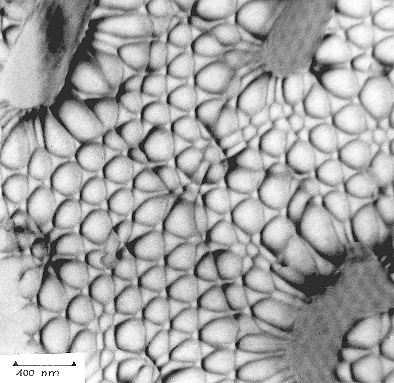
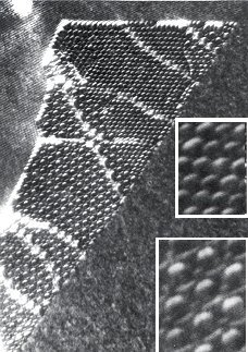
The structure will be much more
complicated and serves to illustrate the importance of the grain boundary plane
for given orientations. The picture below is a bright-field TEM
micrograph (obtained under the specific
bright-field conditions that rival
weak-beam resolution
mentioned before) and shows all dislocations present. |
|
|
|
|
|
|
|
This is also an example of what may
happen to you when you sit down at an electron microscope with your specimen
and start to look at it. |
|
You know what to expect (a small
angle twist grain boundary) in general, but now you see fascinating things -
can you understand what you see? |
|
And, in extrapolation, can you
understand what you see if you do not know beforehand what to expect? |
|
|
|
|
|
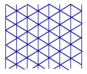
Well, we can understand most of the
structure seen above. Lets construct it step by step |
|
|
|
|
|
|
There must be a network of screw dislocations with b
= a/2<110>. Since three Burgers vectors of this kind are contained in
a given {111} plane, we expect a hexagonal network as shown on the
left. |
|
|
|
|
|
|
|
|
|
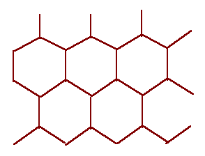
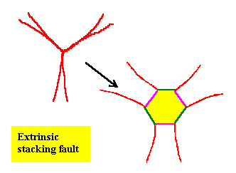
The knots where six dislocations meet can not be
expected to be stable; we would
expect a
splitting leading to the honeycomb pattern illustrated on the left (with a
changed scale for clarity). |
|
|
|
|
|
|
|
|
|
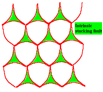
In contrast to the {100} twist boundary, the dislocations now can split
into partial dislocations in the plane of the boundary, we expect that the
dislocations are split in this case. Working through the geometry we see that
everything fits at one knot, it can easily be extended in the way shown. This
optimizes the energy gain by large separations between the partials while at
the same time keeping the stacking fault area small. |
|
The "constricted" knots now look "funny" -
again 6 dislocations meet at one point. Can we split the knot to
something more favorable? |
|
|
|
|
|
|
|
|
|
Indeed, we can, as shown on the left. However, we only can do this by introducing more Shockley
dislocations and extrinsic stacking faults |
|
|
|
|
|
|
|
|
|
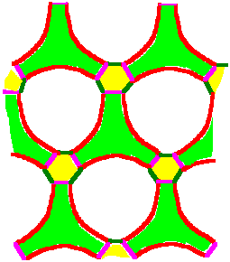
Putting everything together we obtain a network of Shockley
dislocations that corresponds exactly to what we see in the regular parts of
the micrograph above. The exact geometry, of course, depends mainly on the
stacking fault energies - here we may find differences if we would look at
similar grain boundaries in other fcc materials. |
|
|
|
|
|
|
It remains to explain the
various non-regularities of the picture. |
|
|
Most conspicuous are the large "blobs"
with just a trace of some hexagonal structure. They are simply
SiO2 precipitates left over from the welding process; the
hexagonal structures are Moirée
patterns that always appear whenever two regular structures are put on
top of each other. |
|
The other irregularities are formed
by a superposition of: |
|
|
A few edge dislocations to accommodate some tilt
component. |
|
|
Dislocations that moved from somewhere in the
crystal into the grain boundary where they were caught and incorporated into
the network. These dislocations are called extraneous or
extrinsic grain boundary
dislocations because they are not an integral part of the grain
boundary structure. |
|
|
Dislocations needed to accommodate steps, i.e.
changes of the grain boundary plane measuring a few atomic distances. |
|
It is not always clear or easily
analyzed exactly what it is that you see. Especially the connection between
steps and intrinsic or extrinsic dislocation is, in general, quite complicated,
because on the one side most, but not all grain boundary dislocations
automatically introduce steps, while on the other side most, but not all steps
introduce dislocations. We will deal with that matter in more detail when
dealing with phase
boundaries. |
|
But we are not yet done with the low-angle twist
boundary on {111}. The micrograph above shows only part of the
structure. The micrograph below shows more: |
|
|
|
|
|
|
The lower inset shows a magnified view of the
network from the lower half of the boundary; the upper inset from the upper
half. (Click on the picture for an enlargement and
more information), |
|
Whereas the lower part shows the network discussed above, the
upper part shows something new: A rather simple network with reduced spacing.
Detailed analysis reveals that the dislocations in the upper part have Burgers
vectors b = a/6<112>, but they are not proper
Shockley partials, because there are no stacking faults between the
dislocations. |
|
They are rather dislocations in the DSC lattice of a
Σ = 3 boundary - in other words, the low
angle twist boundary has split into two twin boundaries with a superimposed
dislocation network in one of the twin boundaries. |
|
We may ask: Why? And in which twin boundary are the
dislocations? Why are they not in the perfect lattice between the
boundaries? |
|
|
|
|
|
|
It seems to ever end. But in order not to have too
much detail in the main backbone part,
these complications will be
discussed in an advanced section. |
|
|
© H. Föll