|
First we will take a close look at
some small angle grain boundaries in Silicon. Whereas they are the most simple
boundaries imaginable, they are still complex enough to merit some attention.
They are also suitable to demonstrate a few more essential properties of grain
boundary dislocations. |
|
 |
Lets first look at a pure tilt
boundary as outlined in the preceding paragraph. Below is shown how edge
dislocations can accommodate the misfit relative to the Σ = 1 orientation (for a boundary plane that contains
the dislocations lines). |
|
|
|
|
|
|
|
The distance d
between the dislocations is for small tilt angles α as before
given by |
| |
|
|
|
| |
|
|
This is a simple version of a general relation
betwen Burgers vectors and misorientation in small angle grain boundaries
called Franks
formula
(more correctly Frank-Bilby formula). |
|
|
|
|
In real life it looks slightly more complicated -
but not much: |
|
|
|
|
|
|
|
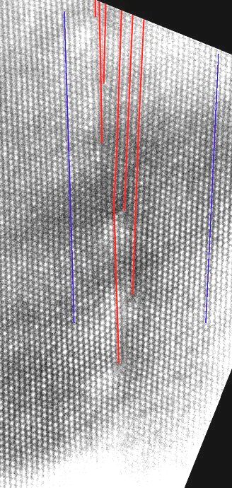
This is an early HRTEM of a small angle tilt boundary
in Si. The red lines mark the edge dislocations, the blue lines indicate
the tilt angle. |
|
This picture nicely illustrates that we have indeed a Σ1 relationship in the area between the dislocations,
i.e. a perfect crystal. The dislocations are not all in a row, but that does
not really matter. |
|
|
|
|
Next, we look at twist
boundaries. |
|
|
These and some of the other boundaries were
artificially produced to study the structure. Two specimens of
Si with a desired orientation relationship were placed on top of each
other and "sintered" or "welded" together at high
temperatures. This process, first called "sintering" is now known as
"waferbonding" and used for
technical applications. |
|
|
The result for a slight twist
between {100} planes is shown in the next picture: |
|
|
|
|
|
|
|
|
|
|
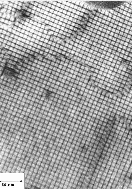
This is a remarkable picture. As
ascertained by contrast analysis, it shows a square network of pure screw dislocations. The picture is remarkable
not only because it shows a rather perfect square network of screw
dislocations, but because it is obviously a
bright
field TEM micrograph, however with a resolution akin to
weak-beam
conditions. |
|
|
Pictures like this one are obtained by orienting
the specimen close to a {100} (or, in other cases, {111})
orientation thus exciting many reflections weakly. All dislocations are then
imaged, but the detailed contrast mechanism causing the superb resolution is
not too clear. |
|
Lets first find out why a network like this can
produce the required twist. We do this in reverse order, i.e. we will construct
a screw dislocation network in a perfect crystal and see what it does. |
|
|
We start by looking at {100} lattice planes
below and above the (future) grain boundary plane. They are exactly on top of
each other, we obtain a (trivial) picture of a formal low-angle twist boundary
with twist angle α = 0o. |
|
|
|
|
|
|
|
|
|
|
|
Now we introduce two screw dislocations running
from left to right. Referring to the
same
kind of picture in chapter 5, we see that the lattice planes below the
screw dislocations are bent to the right (blue lines), above the screw
dislocations to the left: |
|
|
|
|
|
|
|
|
|
|
|
With many dislocations, the average orientation of
the lattice planes below the small angle grain boundary will rotate to the
right, above to the left. The combined effect is shown below. |
|
|
|
|
|
|
|
|
|
|
If we want to rotate not just one set of lattice
planes, but all of the top part of the crystal, we need at least a second set
of screw dislocations. This produces a screw dislocation network of the kind
shown in the TEM micrograph above. |
|
|
The relation between the twist angle α and the dislocation spacing d is again
a simple version of the general case given in Franks formula: |
|
|
|
|
|
|
|
|
|
|
|
A detailed drawing of this dislocation network
structure can be viewed in the link. |
|
|
With luck, it is possible to image the lattice
plane in a HRTEM micrograph. The link shows examples - the only
HRTEM image of screw
dislocations obtained so far. |
|
The exact geometry of the network for the same
twist angle α in an arbitrary twist boundary depends on many
factors: |
|
|
The twist angle
α which determines the spacing between
the dislocations. For Σ = 1 boundaries it
simply the twist angle itself, for arbitrary boundaries it is the twist angle
needed to bring the boundary to the closest low Σ orientation |
|
|
The Burgers
vectors of the dislocations. Even in small-angle grain boundaries
they could be perfect, or split into partials. In arbitrary boundaries they
must be grain boundary dislocations with a Burgers vector of the proper
DSC lattice. Note that a network of grain
boundary screw dislocations simply superimposes some twist to
whatever orientation the boundary has without those dislocations. |
|
|
The type of the
dislocations. For an arbitrary twist plane, the Burgers vectors of
the possible dislocations are not necessarily contained in the grain boundary
plane; the required pure screw dislocations do not exist. In this case mixed
dislocations must be used with a component of the Burgers vector in the grain
boundary plane. |
|
|
The symmetries
of the two crystal planes in contact at the grain boundary - even low-angle
twist boundaries with a twist around the <100> axis can be joined
on planes other than {100}. |
|
|
The complications that may arise
because the (perfect) dislocations split into
partials. Obviously, that has not happened in the case shown above.
The reason most likely is that the splitting would have to be on two different
{111} planes inclined to the boundary plane (look at your Thompson
tetrahedron!) which leads to very unfavorable knot configurations. Since the
distance between dislocations is of the same order of magnitude as the typical
distance between partials, we do not observe splitting into partials or
dissociation of the knots. |
|
We now can understand the very regular square
network shown in the picture above - it is
really about the most simple structure imaginable. |
|
|
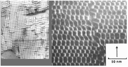
But we still need to explain the
interruptions in the network; the lines along which the net is shifted. In
fact, to see a very regular network like this you must be pretty lucky; more
often than not often (artificially) made twist grain boundaries look like
this: |
|
|
|
|
|
|
|
|
|
|
|
Both pictures show the result of the attempt to
make a pure twist boundary. Whereas the left one still looks like the
picture above - just with more interruption of
the network - the right one does not convey the impression of a square network
at all. |
|
|
The answer is that these grain boundaries must
accommodate more that just a pure twist: There is also a tilt component and the
plane of the grain boundary is not exactly {100}. We will pick up this
subject again in the next paragraph;
more information about the
right-hand side picture can be found in the link. |
|
|
|
© H. Föll